CNS*2021 Online: Tutorials
Tutorials are intended as introductions into main methodologies of various fields in computational neuroscience. This year, CNS tutorials offer introductory full day courses covering a wide range of different topics as well as specialized half day tutorials all taking place over the week preceding the event. Tutorials are particularly tailored for early stage researchers as well as researchers entering a new field in computational neuroscience. Tutorials are grouped into the following categories: Software Tutorials on Mon/Tues June 28/29th, Satellite Tutorials on Wed-Fri June 30th-July 2nd, Tutorials and Showcases on July 3rd.
For inquiries related to tutorials, please contact the tutorials organizer: [email protected].
Software tutorials, June 28-29
Satellite tutorials, June 30 - July 2
| Title | Lecturers | Reference | Web |
|---|
| Introducing the Arbor simulator: what’s new and hands-on tutorial |
Brent F. B. Huisman (Jülich Supercomputing Centre (JSC), Juelich, Germany) |
SA1 |
Link |
| Building, validating, analyzing, and simulating standardized computational models using NeuroML |
Dr. Ankur Sinha (University College London, UK), Angus Silver (University College London, UK), and Padraig Gleeson (University College London, UK) |
SA2 |
Link |
| Signal processing and data analysis in Matlab |
Dr. Cengiz Gunay (SST, Georgia Gwinnett College, USA) |
SA3 |
Link |
| Methods from Data Science for Model Simulation, Analysis, and Visualization |
Dr. Cengiz Gunay (SST, Georgia Gwinnett College, USA) and Dr. Anca Doloc-Mihu (SST, Georgia Gwinnett College, USA) |
SA4 |
Link |
| From synapses to behavior – using open data, tools, and models from the Allen Institute in computational neuroscience |
Anton Arkhipov, Luke Campagnola, Kael Dai, Saskia de Vries, Marina Garrett, Nathan Gouwens, Alex Piet, and Josh Siegle (Allen Institute, USA) |
SA5 |
Link |
Tutorials, July 3
| Title | Lecturers | Reference | Web |
|---|
| Building biophysically detailed neuronal models from molecules to networks with NEURON and NetPyNE |
Dr. Robert A McDougal (Yale University, USA), Dr. Adam JH Newton (Yale University, USA), Dr. Salvador Dura-Bernal (SUNY Downstate, USA), and Dr. William W Lytton (SUNY Downstate, USA) |
T1 |
Link |
| Recurrent Neural Networks dynamics and software implementation with Keras and TensorFlow |
Dr. Cecilia Jarne (University of Quilmes and CONICET Bernal, Argentina) |
T2 |
Link |
| Understanding early visual receptive fields from efficient coding principles |
Dr. Li Zhaoping (University of Tuebingen, Germany) |
T3 |
Link |
| Interactive design and analysis of point neuron spiking networks with synaptic plasticity using NEST Simulator |
Charl Linssen (JARA-Institute, Jülich, Germany), Barna Zajzon, Sebastian Spreizer (University of Trier, Germany), Jasper Albers, and Dennis Terhorst |
T4 |
Link |
Showcases, July 3
| Title | Lecturers | Reference | Web |
|---|
| GPU enhanced Neuronal Networks – GeNN |
Dr. Thomas Nowotny (University of Sussex, UK) and James C Knight (University of Sussex, UK) |
S1 |
TBA |
| Simulating spiking neural networks with the Brian 2 simulator |
Marcel Stimberg (Vision Institute/Sorbonne University, Paris, France) and Dr. Dan Goodman (Imperial College, London, UK) |
S2 |
Link |
| CompNeuroFedora - a community-developed Free/Open Source Operating System for computational neuroscience |
Dr. Ankur Sinha (University College London & Fedora project, London, UK) |
S3 |
Link |
| Introduction to the Brain Dynamics Toolbox |
Dr. Stewart Heitmann (Victor Chang Cardiac Research Institute, Australia) |
S4 |
Link |
| Tools for Leveraging Feature-Based Time-Series Analysis to Characterize Neural Dynamics |
Dr. Ben D Fulcher (The University of Sydney, Australia) |
S5 |
TBA |
| Correcting for Autocorrelation-induced Bias in Linear-dependence Measures: with Applications to Functional Connectivity Analysis |
Dr. Oliver Cliff (The University of Sydney, Australia) |
S6 |
TBA |
Descriptions
SO1: Effective use of Bash
Description of the tutorial
The purpose of this tutorial is to introduce participants to the tools they need in order to comfortably and confidently work with a Unix/Linux command line terminal. Unlike graphical user interfaces, which are often self-explanatory or have obvious built-in help options, the purely text-based nature of a command line terminal can be intimidating and confusing to novice users. Yet, once mastered, the command line offers more flexibility and smoother workflows for many tasks, while being entirely irreplaceable for things such as cluster access.
In this tutorial, we aim to introduce participants to the concepts and tools they need to confidently operate within a Unix/Linux command line environment. In particular, the tutorial is developed for Bash (as per the title), which should cover most Linux and MacOS* use cases. We hope to provide participants with a firm understanding of the basics of using a shell, as well as an understanding of the advantages of working from a command line.
The tutorial is aimed not only at novices who have rarely or never used a command line, but also at occasional or even regular users of bash who seek to expand or refresh their repertoire of everyday commands and the kinds of quality-of-life tricks and shortcuts that are rarely covered on StackExchange questions. * While MacOS has switched from bash to zsh as its default shell, zsh's operation is sufficiently similar for the purposes of this tutorial.
Prerequisites
A working copy of bash; participants on Linux and MacOS are all set.
Participants on Windows have several options to get hold of a bash environment without leaving familiar territory:
- Install Git for Windows (https://gitforwindows.org/), which includes a Git Bash emulation with most of the standard tools you might expect in a Linux/Unix environment, plus of course Git.
- Alternatively, enable WSL2 (https://docs.microsoft.com/en-us/windows/wsl/install-win10#install-the-windows-subsystem-for-linux) and install Ubuntu (https://www.microsoft.com/en-gb/p/ubuntu/9nblggh4msv6) as a virtual machine hosted by Windows. Somewhat ironically, this requires at least one use of a command line terminal (though not bash); on the upside, the Linux-on-Windows experience can be a smooth and safe first step into Linux territory.
Back to top
SO2: Effective use of Git
- Ankur Sinha (SilverLab at University College London, London, UK).
Description of the tutorial
Version control is a necessary skill that users writing any amount of code should possess. Git is a popular version control tool that is used ubiquitously in software development.
This hands-on session is aimed at beginners who have little or no experience with version control systems and Git. It will introduce the basics of version control and walk through a common daily Git workflow before moving on to show how Git is used for collaborative development on popular Git forges such as GitHub. Finally, it will show some advanced features of Git that aid in debugging code errors.
Prerequisites
The session is intended to be a hands-on session, so all attendees will be expected to run Git commands. A working installation of Git is, therefore, required for this session. We will use GitHub as our Git remote for forking and pull/merge requests. So a GitHub account will also be required.
- Linux users can generally install Git from their default package manager:
- Fedora: sudo dnf install git
- Ubuntu: sudo apt-get install git
- Windows users should use Git for Windows (https://gitforwindows.org/).
- MacOS users should use brew to install git: brew install git.
More information on installing Git can be found on the project website: https://git-scm.com/
Back to top
SO3: Python for beginners
Description of the tutorial
Python is amongst the most widely used programming languages today, and is increasingly popular in the scientific domain. A large number of tools and simulators in use currently are either implemented in Python, or offer interfaces for their use via Python. Python programming is therefore a very sought after skill in the scientific community.
This tutorial is targeted towards people who have some experience with programming languages (e.g. MATLAB, C, C++, etc), but are relatively new to Python. It is structured to have you quickly up-and-running, giving you a feel of how things work in Python. We shall begin by demonstrating how to setup and manage virtual environments on your system, to help you keep multiple projects isolated. We'll show you how to install Python packages in virtual environments and how to manage them. This will be followed by a quick overview of very basic Python constructs, leading finally to a neuroscience-themed project that will give you the opportunity to bring together various programming concepts with some hands-on practice.
Prerequisites
- shell (participants on Linux and MacOS are all set; see below for Windows users)
- Python 3.6.9 or higher (see below for info on installation)
Participants on Windows have several options to get hold of a shell environment without leaving familiar territory:
- Install Git for Windows (https://gitforwindows.org/), which includes a Git Bash emulation with most of the standard tools you might expect in a Linux/Unix environment, plus of course Git.
- Alternatively, enable WSL2 (https://docs.microsoft.com/en-us/windows/wsl/install-win10#install-the-windows-subsystem-for-linux) and install Ubuntu (https://www.microsoft.com/en-gb/p/ubuntu/9nblggh4msv6) as a virtual machine hosted by Windows. This Linux-on-Windows experience can be a smooth and safe first step into Linux territory.
You will find several resources online for info on installing Python. e.g. https://realpython.com/installing-python/.
Back to top
SA1: Introducing the Arbor simulator: what’s new and hands-on tutorial
- Brent F.B. Huisman (Institute for Advanced Simulation (IAS), Jülich Supercomputing Centre (JSC), Forschungszentrum Jülich (FZJ), Juelich, Germany)
Description of the tutorial
Arbor is a performance portable library designed to handle very large and computationally intensive simulations of networks of multi-compartment neurons. At the same time, Arbor is designed to be easy to use and understand, so that also beginners to computational neuroscience can get up to speed quickly. Furthermore, Arbor aims to prepare computational neuroscientists to take advantage of HPC architectures. Whether your model is large or small, Arbor is able to optimize and compute your result on almost any current and future hardware.
In this session, we’ll first introduce the Arbor simulator library. We will go into questions such as:
- What is portability and why is it relevant to a computational neuroscientist?
- What is performance portability and why is it relevant to a computational neuroscientist?
- How did the above considerations impact Arbors design?
- How did it impact Arbors API design, which is to say: how easy to use is all this?
- What’s new in Arbor? Current developments include performance improvements for gap junctions, file format compatibility, the Arbor GUI and more!
After the introduction, it is time for a hands-on session where Arbor is used to:
- construct a morphological cell,
- construct a network,
- configure how the simulation is run (single core, multi core, GPU, or MPI, up to you!),
- produce results!
Participating in the tutorial assumes that attendees are comfortable using the Python programming language. No prior knowledge of Arbor or constructing neuroscientific simulations is required.
Useful links
Main website: arbor-sim.org
Documentation: docs.arbor-sim.org
Tutorials: docs.arbor-sim.org/en/latest/tutorial/
Preparation
Although preparation is not required, having a look throughthe Arbor documentation beforehand can help you get the most out of this tutorial. If you wish to run the tutorial on your own machine, make sure you have Python installed (v3.6 or higher) and have installed the `arbor` and `seaborn` packages through `pip`, e.g. `pip install arbor seaborn`.
Note: Windows users are supported through WSL and WSL only at this time.
Back to top
SA2: Building, validating, analyzing, and simulating standardized computational models using NeuroML
- Ankur Sinha (University College London, London, UK)
- Angus Silver (University College London, London, UK)
- Padraig Gleeson (University College London, London, UK)
Description of the tutorial
Biologically detailed neuron and network models remain important tools in neuroscience research. A number of simulation platforms are available to users to develop, simulate, and analyse computational models. Whereas the availability of multiple simulation platforms allows for efficient modelling, the specialised simulator specific modelling languages and input formats these tools use limits interoperability, accessibility, cross-simulator validation, and the reuse of modelling components. NeuroML was developed to overcome these limitations. It is a well established, international, collaborative initiative that develops the NeuroML model description standard and its companion tools. NeuroML allows users to easily develop, validate, analyse, share their models. Additionally, as a simulator independent format, NeuroML also allows the simulation of models across multiple simulation engines.
In this tutorial, targeted at both novice and advanced users, we will discuss the aforementioned benefits of using NeuroML using a series of hands-on sessions. Beginning with a brief introduction of the NeuroML standard and its design principles, we will walk through computational models at different levels of complexity, from single compartment point neuron models to networks of more biophysically realistic and complex multi-compartmental neuron models. In each session, we will show how the NeuroML Python tools (pyNeuroML, libNeuroML) can be used to build, validate, analyse, and simulate models.
No prior knowledge of NeuroML is expected to attend this session. While users can install the necessary software with ease following the steps listed in the NeuroML documentation, they can also use the Jupyter Notebooks included in the NeuroML documentation or on Open Source Brain for this tutorial. Since this tutorial will use the NeuroML Python tools, a basic knowledge of the Python programming language is required along with some knowledge of computational modelling.
Documentation for NeuroML can be found at https://docs.neuroml.org.
Background reading and software tools
Attendees may install these on their local computers. However, they may also use the Jupyter note books provided in the NeuroML documentation on Binder or Google Colaboratory for the tutorial.
While no prior knowledge of NeuroML is assumed, interested attendees may read the following in preparation:
- P. Gleeson et al., “NeuroML: A Language for Describing Data Driven Models of Neurons and Networks with a High Degree of Biological Detail,” PLoS Computational Biology, vol. 6, no. 6, Art. no. 6, 2010, doi: 10.1371/journal.pcbi.1000815.
- M. Vella et al., “libNeuroML and PyLEMS: using Python to combine procedural and declarative modeling approaches in computational neuroscience.,” Frontiers in neuroinformatics, vol. 8, p. 38, 2014, doi: 10.3389/fninf.2014.00038.
- R. C. Cannon et al., “LEMS: a language for expressing complex biological models in concise and hierarchical form and its use in underpinning NeuroML 2,” Frontiers in Neuroinformatics, vol. 8, 2014, doi: 10.3389/fninf.2014.00079.
The NeuroML Documentation at https://docs.neuroml.org provides an excellent starting point for NeuroML users and developers.
Schedule of tutorial sessions:
(Timings are approximate and may vary depending on how interactive the attendees are etc.)
- Introduction to NeuroML (~45 minutes)
- Break (~15 minutes)
- Hands on session #1: (~45 minutes)
- Break + questions (~15 minutes)
- Hands on session #2: (~45 minutes)
- Break + questions (~15 minutes)
- Hands on session #3: (~45 minutes)
- Break + questions (~15 minutes)
- Hands on session #4: (~45 minutes)
- Concluding remarks (~15 minutes)
Back to top
SA3: Signal processing and data analysis in Matlab
- Cengiz Gunay (School of Science and Technology, Georgia Gwinnett College, USA)
Description of the tutorial
Matlab (Mathworks, Natick, MA) is a popular computing environment that offers an alternative to more advanced environments with its simplicity, especially for those less computationally inclined or for collaborating with experimentalists. In this tutorial, we will focus on the following tasks in Matlab:
- Signal processing of recorded or simulated traces (e.g., filtering noise, spike and burst finding in single-unit intracellular electrophysiology data in current-clamp, and extracting numerical characteristics);
- analyzing tabular data (e.g. obtained from Excel or from the result of other analyses);
- plotting and visualization.
For all of these, we will take advantage of the PANDORA toolbox, which is an open-source project that has been proposed for analysis and visualization ( RRID: SCR_001831, [1]). PANDORA was initially developed for managing and analyzing brute-force neuronal parameter search databases. However, it has proven useful for various other types of simulation or experimental data analysis [2-7]. PANDORA’s original motivation was to offer an object-oriented program for analyzing neuronal data inside the Matlab environment, in particular with a database table-like object, similar to the “dataframe” object offered in the R ecosystem and the pandas Python module. PANDORA offers a similarly convenient syntax for a powerful database querying system. A typical workflow would constitute of generating parameter sets for simulations, and then analyze the resulting simulation output and other recorded data, to find spikes and to measure additional characteristics to construct databases, and finally analyze and visualize these database contents. PANDORA provides objects for loading datasets, controlling simulations, importing/exporting data, and visualization. In this tutorial, we use the toolbox’s standard features and show how to customize them for a given project.
Software tools:
References:
- Günay et al. 2009 Neuroinformatics, 7(2):93-111. doi: 10.1007/s12021-009-9048-z
- Doloc-Mihu et al. 2011 Journal of biological physics, 37(3), 263–283. doi:10.1007/s10867-011-9215-y
- Lin et al. 2012 J Neurosci 32(21): 7267–77
- Wolfram et al. 2014 J Neurosci, 34(7): 2538–2543; doi: 10.1523/JNEUROSCI.4511-13.2014
- Günay et al. 2015 PLoS Comp Bio. doi: 10.1371/journal.pcbi.1004189
- Wenning et al. 2018 eLife 2018;7:e31123 doi: 10.7554/eLife.31123
- Günay et al. 2019 eNeuro, 6(4), ENEURO.0417-18.2019. doi:10.1523/ENEURO.0417-18.2019
Back to top
SA4: Methods from Data Science for Model Simulation, Analysis, and Visualization
- Cengiz Gunay (School of Science and Technology, Georgia Gwinnett College, USA)
- Anca Doloc-Mihu (School of Science and Technology, Georgia Gwinnett College, USA)
Description of the tutorial
Computational neuroscience projects often involve large number of simulations for parameter search of computer models, which generates large amount of data. With the advances in computer hardware, software methods, and cloud computing opportunities making this task easier, the amount of collected data has exploded, similar to what has been happening in many fields. High performance computing (HPC) methods have been used in the computational neuroscience field for a while. However, use of novel data science and big data methods are less frequent.
In this tutorial, we will review tools already established in the big data field and demonstrate their usefulness in computational neuroscience workflows, focusing on Apache Spark (https://spark.apache.org/). Spark is a distributed computing framework used either for model simulation or for post-processing and analysis of the generated data. The tutorial will also have a session focusing on creating interactive visualizations. We will review novel web-based interactive notebook technologies based on Javascript (Observable) and Python (Jupyter).
Software tools
- Apache Spark
- Observable
- Jupyter
Expected knowledge/materials
- Some familiarity with Python, Javascript, HTML
- Command line usage for accessing remote servers
- For the visualization session: Google Account suggested to use the online Jupyter notebook service at Colab
Back to top
SA5: From synapses to behavior – using open data, tools, and models from the Allen Institute in computational neuroscience
- Anton Arkhipov (Mindscope Program at the Allen Institute, Seattle, USA)
- Luke Campagnola (Allen Institute for Brain Science, Seattle, USA)
- Kael Dai (Mindscope Program at the Allen Institute, Seattle, USA)
- Saskia de Vries (Mindscope Program at the Allen Institute, Seattle, USA)
- Marina Garrett (Mindscope Program at the Allen Institute, Seattle, USA)
- Nathan Gouwens (Allen Institute for Brain Science, Seattle, USA)
- Alex Piet (Mindscope Program at the Allen Institute, Seattle, USA)
- Josh Siegle (Mindscope Program at the Allen Institute, Seattle, USA)
Description of the tutorial
The Allen Institute recently released multiple free resources focusing on the structure and function of brain circuits. These resources include data, associated analysis software, and models integrating the data to enable bio-realistic simulations. They provide a powerful ecosystem for a new generation of analyses, theory, and modeling in computational neuroscience.
We will introduce several of these resources in a series of 1-hour sessions. Each session will include a scientific introduction for the resource and an online demonstration of accessing and analyzing the data.
The resources covered will include:
- PatchSeq Characterization of Cell Types [1]. This dataset describes >4,000 cells from the mouse and human cortex. Intrinsic electrophysiological properties, morphologies, and transcriptomic profiles are measured from the same neurons, and types are assigned to those cells based on different properties. https://portal.brain-map.org/explore/classes/multimodal-characterization
- Synaptic Physiology [2]. This dataset describes >1,500 synapses from mouse and human cortex. Measured properties include connectivity, synaptic strength, variance, and short-term plasticity. Cells are classified by their layer, transgenic markers, morphology, and intrinsic physiological features, allowing comparisons between many cell subclasses. http://portal.brain-map.org/explore/connectivity/synaptic-physiology
- Visual Coding 2-photon [3]. This dataset contains 2-photon calcium imaging data that surveys visual responses across 6 cortical areas, 4 cortical layers, and 14 transgenically defined cell populations. Activity was imaged in awake mice in response to a variety of stimuli, while tracking the mouse’s running speed and pupil size in each session. https://portal.brain-map.org/explore/circuits/visual-coding-2p
- Visual Coding Neuropixels [4]. This dataset includes spiking activity from neurons recorded across more than dozen brain regions while mice viewed diverse visual stimuli. Each experiment includes spikes from hundreds of simultaneously recorded neurons, as well as local field potentials. https://portal.brain-map.org/explore/circuits/visual-coding-neuropixels
- Visual Behavior [5]. This dataset contains 2-photon calcium imaging recordings from transgenically defined cell populations across two cortical regions while mice perform a visual change detection task. Each experiment includes the activity of individual neurons and behavioral data. https://portal.brain-map.org/explore/circuits/visual-behavior-2p
- Bio-realistic model of the mouse primary visual cortex [6]. The model integrates data from the Allen Institute and the literature on composition, connectivity, and in vivo activity of cortical circuits. https://portal.brain-map.org/explore/models/mv1-all-layers
Software tools
Background Reading
- Gouwens NW, Sorensen SA, Baftizadeh F, Budzillo A, Lee BR, Jarsky T, et al. Integrated Morphoelectric and Transcriptomic Classification of Cortical GABAergic Cells. Cell. 2020;183: 935-953.e19. doi:https://doi.org/10.1016/j.cell.2020.09.057
- Campagnola L, Seeman SC, Chartrand T, Kim L, Hoggarth A, Gamlin C, et al. Connectivity and Synaptic Physiology in the Mouse and Human Neocortex. bioRxiv. 2021; 2021.03.31.437553. doi:10.1101/2021.03.31.437553
- de Vries SEJ, Lecoq JA, Buice MA, Groblewski PA, Ocker GK, Oliver M, et al. A large-scale standardized physiological survey reveals functional organization of the mouse visual cortex. Nat Neurosci. 2020;23: 138–151. doi:10.1038/s41593-019-0550-9
- Siegle JH, Jia X, Durand S, Gale S, Bennett C, Graddis N, et al. Survey of spiking in the mouse visual system reveals functional hierarchy. Nature. 2021. doi:10.1038/s41586-020-03171-x
- Garrett M, Manavi S, Roll K, Ollerenshaw DR, Groblewski PA, Ponvert ND, et al. Experience shapes activity dynamics and stimulus coding of VIP inhibitory cells. Elife. 2020;9. doi:10.7554/eLife.50340
- Billeh YN, Cai B, Gratiy SL, Dai K, Iyer R, Gouwens NW, et al. Systematic Integration of Structural and Functional Data into Multi-scale Models of Mouse Primary Visual Cortex. Neuron. 2020;106: 388-403.e18. doi:10.1016/j.neuron.2020.01.040
Schedule:
Wednesday, June 30, 2021:
- 11:30 am – 11:45 am EST (8:30 am – 8:45 am PT) - Introduction
- 11:45 am – 12:45 pm EST (8:45 am – 9:45 am PT) - Synaptic Physiology (Luke Campagnola)
- 12:45 pm – 1:00 pm EST (9:45 am – 10:00 am PT) - Break
- 1:00 pm – 2:00 pm EST (10:00 am – 11:00 am PT) - Visual Coding 2-photon (Saskia de Vries)
- 2:00 pm – 3:00 pm EST (11:00 am – 12:00 pm PT) - Visual Coding Neuropixels (Josh Siegle)
Thursday, July 1, 2021
- 11:30 am – 11:45 am EST (8:30 am – 8:45 am PT) - Introduction
- 11:45 am – 12:45 pm EST (8:45 am – 9:45 am PT) - PatchSeq (Nathan Gouwens)
- 12:45 pm – 1:00 pm EST (9:45 am – 10:00 am PT) - Break
- 1:00 pm – 2:00 pm EST (10:00 am – 11:00 am PT) - Visual Behavior (Alex Piet)
- 2:00 pm – 3:00 pm EST (11:00 am – 12:00 pm PT) - Bio-realistic model of the mouse primary visual cortex (Anton Arkhipov and Kael Dai)
Back to top
T1: Building biophysically detailed neuronal models from molecules to networks with NEURON and NetPyNE
- Robert A McDougal (Yale University, USA)
- Adam JH Newton (Yale University, USA)
- Salvador Dura-Bernal (SUNY Downstate, USA)
- William W Lytton (SUNY Downstate, USA)
Description of the tutorial
Understanding brain function requires characterizing the interactions occurring across many temporal and spatial scales. Mechanistic multiscale modeling aims to organize and explore these interactions. In this way, multiscale models provide insights into how changes at molecular and cellular levels, caused by development, learning, brain disease, drugs, or other factors, affect the dynamics of local networks and of brain areas. Large neuroscience data-gathering projects throughout the world (e.g. US BRAIN, EU HBP, Allen Institute) are making use of multiscale modeling, including the NEURON ecosystem, to better understand the vast amounts of information being gathered using many different techniques at different scales.
This tutorial will introduce multiscale modeling using two NIH-funded tools: the NEURON 8.0 simulator [1], including the Reaction-Diffusion (RxD) module [2,3], and the NetPyNE tool [4]. The tutorial will combine background, examples and hands on exercises covering the implementation of models at four key scales: (1) intracellular dynamics (e.g. calcium buffering, protein interactions), (2) single neuron electrophysiology (e.g. action potential propagation), (3) neurons in extracellular space (e.g. spreading depression), and (4) networks of neurons. For network simulations, we will use NetPyNE, a high-level interface to NEURON supporting both programmatic and GUI specification that facilitates the development, parallel simulation, and analysis of biophysically detailed neuronal circuits. We conclude with an example combining all three tools that links intracellular molecular dynamics with network spiking activity and local field potentials.
Basic familiarity with Python is recommended. No prior knowledge of NEURON or NetPyNE is required. The tutorial will use these tools on the cloud, so no software installation is necessary.
Software tools
References and Background Reading
If you’re new to Python programming, there are many excellent tutorials online. There are Python lectures with exercises and solutions taught by one of us in a summer course last year under “Monday” at https://ycmi.github.io/summer-course-2020/
- Lytton WW, Seidenstein AH, Dura-Bernal S, McDougal RA, Schürmann F, Hines ML. Simulation Neurotechnologies for Advancing Brain Research: Parallelizing Large Networks in NEURON . Neural Comput. 28, 2063–2090, 2016.
- McDougal R, Hines M, Lytton W. (2013) Reaction-diffusion in the NEURON simulator. Front. Neuroinform. 7, 28. 10.3389/fninf.2013.00028.
- Newton AJH, McDougal RA, Hines ML and Lytton WW (2018) Using NEURON for Reaction-Diffusion. Modeling of Extracellular Dynamics. Front. Neuroinform. 12, 41. 10.3389/fninf.2018.00041.
- Dura-Bernal S, Suter B, Gleeson P, Cantarelli M, Quintana A, Rodriguez F, Kedziora DJ, Chadderdon GL, Kerr CC, Neymotin SA, McDougal R, Hines M, Shepherd GMG, Lytton WW. (2019) NetPyNE: a tool for data-driven multiscale modeling of brain circuits. eLife 2019;8:e44494.
Schedule:
All times listed for New York City (EDT):
- 10:00 - 10:30 - Bill Lytton - Overview: Implementing the Conceptual Model
- 10:30 - 11:50 - Robert McDougal - NEURON scripting basics
- 11:50 - 12:00 - coffee break
- 12:00 - 1:00 - Adam Newton - Reaction-Diffusion
- 1:00 - 1:30 - lunch break
- 1:30 - 2:50 - Salvador Dura - NetPyNE GUI-based tutorials
- 2:50 - 3:00 - coffee break
- 3:00 - 4:00 - Salvador Dura - NetPyNE programmatic tutorial
Back to top
T2: Recurrent Neural Networks dynamics and software implementation with Keras and TensorFlow
- Cecilia Jarne (Department of Science and Technology from the University of Quilmes and CONICET Bernal, Buenos Aires, Argentina)
Description of the tutorial
This tutorial will help participants to implement and explore simple neural models using Keras [1]. This year the focus will be on the implementation of Recurrent Neural Network (RNN) to perform temporal tasks. Such models are of great interest to different scientific communities, for example, Computational Neuroscience research and dynamical systems. Open-source frameworks dedicated to Machine Learning, such as Keras [1] and Tensorflow [2], have produced significant changes in the development of technologies that we currently use. One relevant problem that can be approached using them, is how to build the models for the study of dynamical systems and how to extract the relevant information to answer scientific questions of interest related to brain modeling.
The tutorial will include an introduction to modeling, discussion, and hands-on exercises. It will focus on using Keras to develop Neural Networks for rapid prototyping and simulate with TensorFlow [2] as backend. We will study implementations of recurrent neural networks with Keras split into two sections: First, we will introduce the main keys of Recurrent Neural Networks and dynamics, and on the second part, the features of Keras showcasing some examples to run.
Software tools
For this tutorial, you will need basic knowledge of NumPy, SciPy, and matplotlib. To be able to carry out the tutorial we will use google colab (https://colab.research.google.com/) or if you prefer, a laptop with Linux and these libraries installed:
- Python
- Numpy
- SciPy
- Matplotlib
- Scikit learn
- TensorFlow
- Keras
I recommend the following sites where is explained the installation of the following packages that include a set of the named libraries and some additional tools:
References
- Francois Chollet et al. Keras. https://keras.io, 2015
- Martín Abadi, et al. TensorFlow: Large-scale machine learning on heterogeneous systems, 2015.
- https://www.tensorflow.org/install/
- C. Jarne. What you need to know to train recurrent neural networks to make Flip Flops memories and more https://arxiv.org/abs/2010.07858
Schedule:
The first part consists of a Lecture on Recurrent Neural Networks and implementations with Tensorflow and Keras (1.5 or 2 hrs) then, a break of 15 min and finally we will work on jupyter notebooks with google colab to implement simple and guided exercises (1 hrs approximately).
Slides for the Tutorial will be available at the date of the tutorial.
Back to top
T3: Understanding early visual receptive fields from efficient coding principles
- Li Zhaoping (Max Planck Institute for Biological Cybernetics, University of Tübingen, Germany)
Description of the tutorial
Understanding principles of efficient coding can enable you to answer questions such as: why should the input contrast response function of a neuron take its particular form? Why do retinal ganglion cells have center-surround receptive fields? How correlated or decorrelated should the visual responses from different retinal ganglion cells be? Why do receptive fields of retinal ganglion cells increase their sizes in dim light? How could visual coding depend on animal species? Why are color selective V1 neurons less sensitive to visual motion signals? How can one predict the ocular dominance properties of V1 neurons from developmental conditions? How should neurons adapt to changes in visual environment? This tutorial guides you on how to answer such questions. The detailed content can be seen from the titles of the video clips at http://www.lizhaoping.org/zhaoping/EfficientVisualCoding_Playlist.html
Depending on the learning effort invested, the following are possible outcomes after the tutorial:
- participants can get a gist of, or an introduction to, this topic;
- participants can learn enough to collaborate with experts on this topic, whether as an experimentalist collaborating with a theorist/modeler, or as a modeler/theorist collaborating with an experimentalist;
- participants can learn enough to become independent researchers on this topic.
The tutorial material is based largely on chapter 3 (and some of chapter 4) of the textbook “Understanding vision: theory, models, and data” published by Oxford University Press. This book is available in many university libraries (in ebook form, hard copy, or paper back), see http://www.lizhaoping.org/zhaoping/VisionBook.html for more information. Since the video clips are quite detailed, it is also feasible (although less convenient) to learn without having the textbook.
This tutorial has the following parts:
- Before the tutorial day on July 3rd, students should finish watching the video clips listed at http://www.lizhaoping.org/zhaoping/EfficientVisualCoding_Playlist.html. Each video clip is about 10 minutes long, and there are a total of about 45 clips. For best digestion of the materials, try to watch over multiple days or even weeks, and do not watch more than 1 hour of video clips per day on material that are unfamiliar to you.
- Please email me to let me know who you are, and to get into a Discord channel where students can ask each other and me questions, and have chats and discussions, help each other, and network, particularly before the tutorial day.
- On the tutorial day, there will be the following 3 hour-long zoom sessions (the zoom link will be given), with breaks in between:
Please email me at [email protected] for enquiries.
Back to top
T4: Interactive design and analysis of point neuron spiking networks with synaptic plasticity using NEST Simulator
- Charl Linssen (JARA-Institute, Jülich, Germany)
- Barna Zajzon (Jülich Research Centre, Jülich, and RWTH Aachen University, Aachen, Germany)
- Sebastian Spreizer (University of Trier, Germany)
- Jasper Albers (Jülich Research Centre, Jülich, and RWTH Aachen University, Aachen, Germany)
- Dennis Terhorst (Jülich Research Centre, Jülich, and RWTH Aachen University, Aachen, Germany)
Description of the tutorial
NEST Simulator is an established, open-source community software for simulating small and large-scale networks on general-purpose computer hardware. In this workshop, we will explore several tools in the NEST ecosystem that streamline the research and development which is carried out with NEST at its core. To illustrate how these tools can be used in practice, we will work through concrete examples and hands-on exercises, with a special focus on exploring the effects of plasticity and spatial connectivity on the population dynamics and information processing in modular spiking networks.
We begin with an introduction to NEST with a graphical user interface, NEST Desktop, that integrates the whole workflow of instantiating the network and connectivity, simulating the neuronal dynamics, and analyzing the recorded activity data. It supports teaching the concepts and methods of computational neuroscience.
Next, we will explore spike-timing dependent plasticity (STDP), and review some of the empirical observations before looking at two mathematical formalizations in more detail, namely STDP with all-to-all and nearest-neighbour spike pairing, and the triplet STDP rule from. These mathematical models are then expressed in the NESTML modeling language, and instantiated in a 1simple network which is simulated in NEST. We analyse how the parameters of the plasticity rule influence the evolution of synaptic
strength during simulation.
While this tutorial does not assume any prior knowledge of NEST, familiarity with Python is recommended as large parts of the workflow will be controlled from Jupyter notebooks. Code will be provided for all models, and we invite interactive experimentation during and after the tutorial. Participants will be provided access to virtual machines through a browser, courtesy of
HBP/EBRAINS, but all software is open-source and available for installation on local machine by the users.
Software tools
References and Background Reading
- Zajzon, B., Mahmoudian, S., Morrison, A., & Duarte, R. (2019). Passing the message: representation transfer in modular balanced networks. Frontiers in computational neuroscience.
- Pfister JP, Gerstner W (2006). The Journal of Neuroscience 26(38):9673-9682.
Back to top
S1: GPU enhanced Neuronal Networks (GeNN)
- James Knight (University of Sussex, UK)
- Thomas Nowotny (University of Sussex, UK)
Description of the showcase
The GPU enhanced Neuronal Networks (GeNN) software ecosystem originated as a meta-compiler to translate model descriptions of spiking neural networks into efficient CUDA/C++ code for accelerated simulation on Graphical Processing Units (GPUs) [1]. Since its inception, we have continued to develop GeNN by adding support to additional front-end interfaces for convenient use in different settings [4,5] and by developing further optimizations to improve performance [2,3]. Today, GeNN can be used in a large variety of ways (see Figure 1) and for different purposes, ranging from large-scale simulations on high-performance equipment to closed-loop robotic applications using embedded GPU devices.
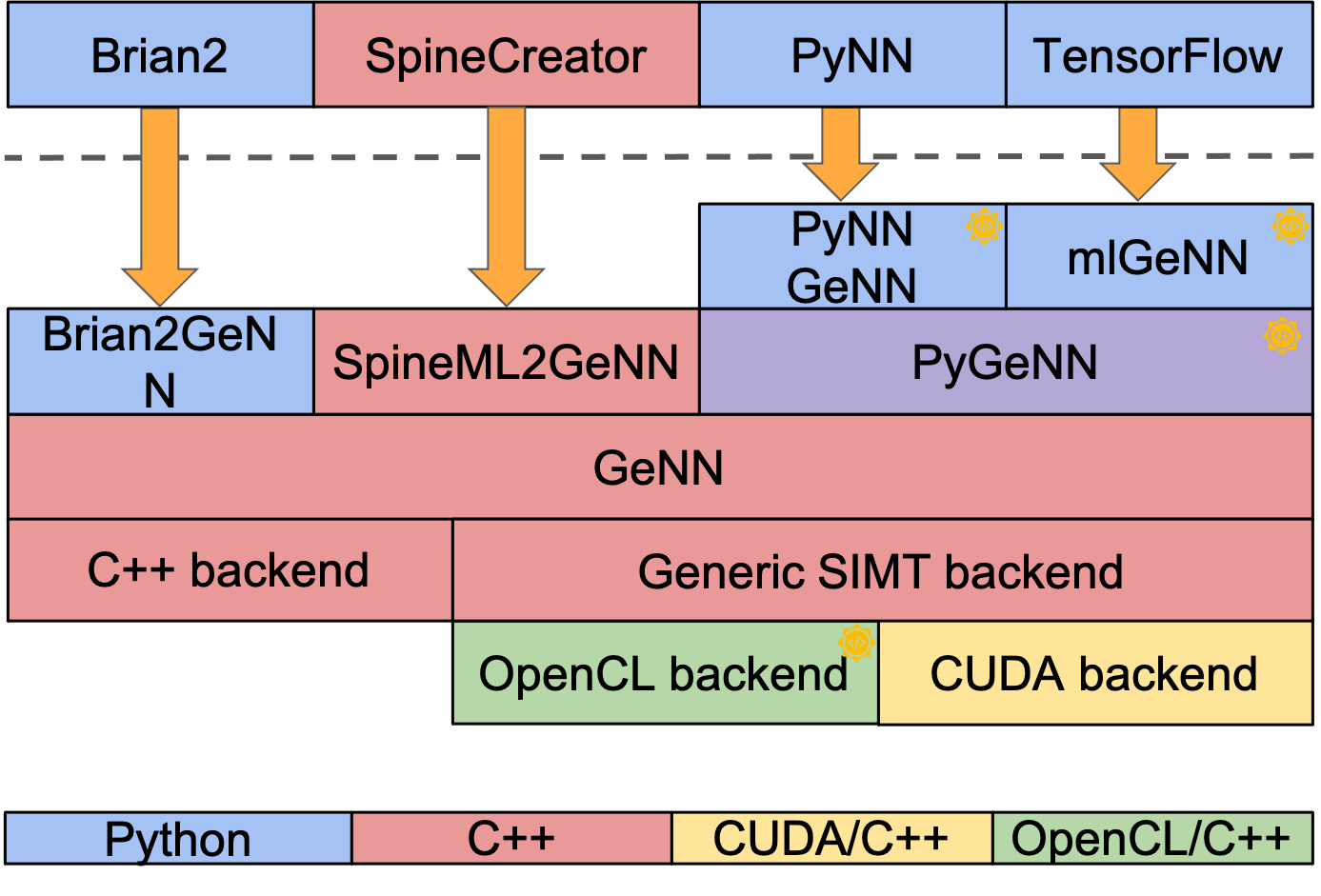
Figure 1: GeNN software ecosystem. Depending on the application and user preference, GeNN can be used through different C++ or Python based interfaces. It supports computing hardware with three different backends - single threaded C++ for traditional CPUs, and OpenCL and CUDA for GPUs and other accelerators.
 = Google Summer of Code sponsored development in collaboration with INCF = Google Summer of Code sponsored development in collaboration with INCF
Software tools
Showcase content
In this showcase we will highlight the use cases of GeNN and some of the popular modes of use. Time permitting we will also discuss some of the most recent advances in scalability and performance, such as procedural connectivity [3].
References and Background Reading
- E. Yavuz, J. Turner and T. Nowotny (2016). GeNN: a code generation framework for accelerated brain simulations. Scientific Reports 6:18854. doi: 10.1038/srep18854
- J. C. Knight, T. Nowotny (2018) GPUs outperform current HPC and neuromorphic solutions in terms of speed and energy when simulating a highly-connected cortical model. Front Neurosci 12:941. doi: 10.3389/fnins.2018.00941
- J. C. Knight and T. Nowotny (2021) Larger GPU-accelerated brain simulations with procedural connectivity. Nat Comput Sci 1(2): 136-42. doi: 10.1038/s43588-020-00022-7, free full text
- J. C. Knight, A. Komissarov, T. Nowotny (2021) PyGeNN: A Python Library for GPU-Enhanced Neural Networks. Frontiers in Neuroinformatics 15: 10. doi: 10.3389/fninf.2021.659005
- M. Stimberg, D. F. M. Goodman, T. Nowotny (2020). Brian2GeNN: accelerating spiking neural network simulations with graphics hardware. Scientific Reports, 10(1), 1–12. Doi: 10.1038/s41598-019-54957-7
Back to top
S2: Simulating spiking neural networks with the Brian 2 simulator
- Marcel Stimberg (Vision Institute / Sorbonne University, Paris, France)
- Dan Goodman (Imperial College, London, UK)
Description of the showcase
The Brian 2 simulator allows scientists to simply and efficiently simulate spiking neural network models using the Python programming language. It provides a highly flexible system for describing almost arbitrary models in mathematical language and referring to physical units. Based on the model description, the simulator transparently generates efficient code in a compiled target language. As a result, Brian 2 overcomes the rigidity of many other simulators while maintaining performance.
In this showcase, we will give examples of Brian’s approach to model description and code generation, and demonstrate how its extensible framework makes it possible to execute the same model on different hardware and software architectures. Finally, we will present and discuss recent advances in the Brian 2 ecosystem, such as a toolbox for automatic fitting of neuronal models to experimental data.
Software tools
References and Background Reading
- Stimberg, M., Brette, R. & Goodman, D. F. Brian 2, an intuitive and efficient neural simulator. eLife 8, e47314 (2019). 10.7554/eLife.47314
- Stimberg, M., Goodman, D. F. M., Benichoux, V. & Brette, R. Equation-oriented specification of neural models for simulations. Frontiers in Neuroinformatics 8, (2014). 10.3389/fninf.2014.00006
Back to top
S3: CompNeuroFedora - a community developed Free/Open Source Operating System for computational neuroscience
- Ankur Sinha (University College London & Fedora project, London, UK)
Description of the showcase
Open Neuroscience is heavily dependent on the availability of Free/Open Source Software (FOSS) tools that support the modern scientific process. While more and more tools are now being developed using FOSS driven methods to ensure free (free to use, study, modify, and share---and so also free of cost) access to all, the complexity of these domain specific tools makes their uptake by the multi-disciplinary neuroscience target audience non-trivial.
The NeuroFedora community initiative aims to make it easier for all to use neuroscience software tools. Using the resources of the FOSS Fedora community, NeuroFedora volunteers identify, package, test, document, and disseminate neuroscience software for easy usage on the general purpose FOSS Fedora Linux Operating System (OS). As a result, users can easily install a myriad of software tools in only two steps: install any flavour of the Fedora OS; install the required tools using the in-built package manager.
To make common computational neuroscience tools even more accessible, NeuroFedora now provides an OS image that is ready to download and use. Users can obtain the CompNeuroFedora OS image from the community website at https://labs.fedoraproject.org/ . They can either install it, or run it “live” from the installation image.
The software showcase will introduce the audience to the NeuroFedora community initiative. It will demonstrate the CompNeuroFedora installation image and the plethora of software tools for computational neuroscience that it includes. It will also give the audience a quick overview of how the NeuroFedora community functions and how they may contribute.
User documentation for NeuroFedora can be found at https://neuro.fedoraproject.org
Back to top
S4: Introduction to the Brain Dynamics Toolbox
- Stewart Heitmann (Victor Chang Cardiac Research Institute, Australia)
Description of the showcase
The Brain Dynamics Toolbox (bdtoolbox.org) is an open-source toolbox for simulating dynamical systems in an interactive graphical interface without the need for graphical programming. It runs in Matlab and solves initial-value problems in the systems of Ordinary Differential Equations (ODEs), Delay Differential Equations (DDEs), Stochastic Differential Equations (SDEs) and Partial Differential Equations (PDEs). The right-hand sides of the equations are defined as custom Matlab functions which are then loaded into the graphical interface for interactive simulation. The hub-and-spoke software architecture allows any combination of plotting tools (display panels) and solver algorithms (ode45, ode23, etc) to be applied to any system of equations with no additional programming effort. Its design fosters rapid prototyping of bespoke dynamical systems. This software showcase aims to introduce the toolbox to a wider audience through a series of real-time demonstrations. The audience will learn how to get started with the toolbox, how to run existing models and how to semi-automate the controls to generate a bifurcation diagram. Further training courses are available from the bdtoolbox.org website.
Background Reading and Software tools
- Brain Dynamics Website. https://bdtoolbox.org
- Heitmann S, Breakspear M (2017-2020) Handbook for the Brain Dynamics Toolbox. QIMR Berghofer Medical Research Institute. 5th Edition: Version 2020, ISBN 978-0-6450669-0-6.
- Heitmann S, Aburn M, Breakspear M (2017) The Brain Dynamics Toolbox for Matlab. Neurocomputing. Vol 315. p82-88. doi:10.1016/j.neucom.2018.06.026.
Back to top
S5: Tools for Characterizing Neural Dynamics using Feature-Based Time-Series Analysis
- Ben Fulcher (School of Physics, The University of Sydney, Australia)
Description of the showcase
Neural dynamics are being measured in unprecedented detail, from microscale neuronal circuits to macroscale population-level recordings. There are myriad ways to quantify useful patterns in neural dynamics—including methods from statistical time-series modeling, the physical nonlinear time-series analysis literature, and methods derived from information theory)—but how do we choose an appropriate tool for a given analysis task? This is typically done subjectively, leaving open the possibility that alternative methods might yield better understanding or performance.
In this software showcase, I will demonstrate tools for extracting informative features from time series, including the Matlab-based hctsa, and similar tools accessible from R, python, and Julia. Focusing on classification problems, I will demonstrate how these tools can be used to automatically distinguish and understand the characteristic properties of different types of experimentally measured (or model simulations of) neural dynamics.
Software tools
References and Background Reading
- B.D. Fulcher, N. S. Jones. hctsa: A computational framework for automated time-series phenotyping using massive feature extraction. Cell Systems 5(5): 527 (2017). https://doi.org/10.1016/j.cels.2017.10.001
- C.H. Lubba et al. catch22: CAnonical Time-series CHaracteristics. Data Min Knowl Disc 33, 1821–1852 (2019). https://doi.org/10.1007/s10618-019-00647-x
Back to top
S6: Correcting for Autocorrelation-induced Bias in Linear-dependence Measures: with Applications to Functional Connectivity Analysis
- Oliver Cliff (School of Physics, The University of Sydney, Australia)
Description of the showcase
Linear dependence measures such as Pearson correlation and Granger causality are used extensively for analysing neuroimaging data from EEG, fMRI, and calcium imaging experiments. However, these statistics are significantly biased by any autocorrelation present in the time series, resulting in spurious associations and statistics that reflect the autocorrelation of each signal rather than a true association.
In this software showcase, I will demonstrate techniques to remove the autocorrelation-induced bias in correlation coefficients, mutual information, and Granger causality through our MATLAB toolkit. Focusing on functional connectivity, I will give a brief overview of the theoretical issues of measuring association between time series, and then illustrate how to infer significant edges in a functional network with fMRI data from the human connectome project resting-state dataset.
Software tools
References and Background Reading
- O. M. Cliff, L. Novelli, B. D. Fulcher, J. M. Shine, and J. T. Lizier. "Assessing the significance of directed and multivariate measures of linear dependence between time series. Physical Review Research 3.1 (2021): 013145.
Back to top
|